From DICOM to MPR (part 4)
This is the fourth part of 5 parts series. Link to part 5.
In the previous installment of this multi-part series of articles we discovered the DICOM standards and how it came to be. The way data are stored according to DICOM and how these data can be extracted and interpreted. We also had a look at the various coordinate systems and how to hop from one to another. Now we will all put this together and render our very first MPR image !
Final results
You can see the final result at this address. An empty canvas should appear on the page. Drag and drop some DICOM instances on it (they should contain at least one full volume). Be careful, Firefox's drag and drop is a little shaky, prefer Chrome here. After a couple of seconds, a coronal view of your volume should appear.
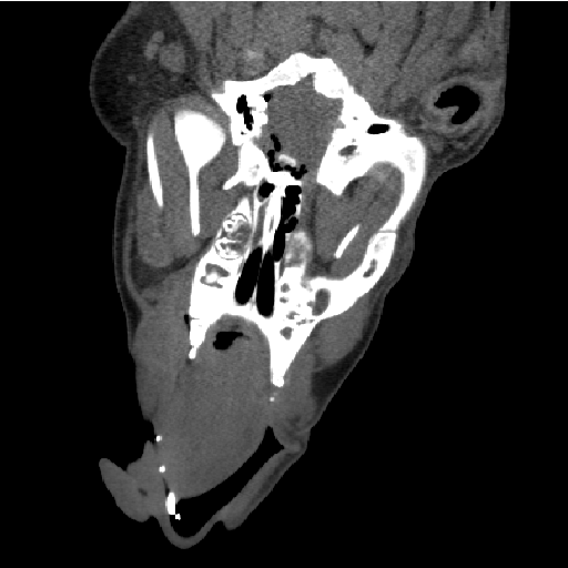
A CT coronal view of a pig.
As previously mentioned, this code aims at simplicity and readability. It does not support all the DICOM variations and quirks. It will work with a well-behaved DICOM format and nothing else. Moreover, it is awfully slow and there are a dozen of optimization opportunities left for the reader as an exercise. An implementation through WebGL is even possible. The only difficulty being to transfer the volume to GPU memory, but the results are impressive, even with tri-linear interpolation ! Maybe the subject of a future article if popular demand is high ;)
Conclusion
Here you go. From DICOM to MPR. The journey was arduous but rewarding. In order to master a technology, one must start from the beginning and be ready to spend much time getting into the details but as a result you gain insight allowing you to produce amazing results.