From DICOM to MPR (part 3)
This is the third part of 5 parts series. Link to part 4.
In the first part of this series we had a look at what DICOM is and how it came to be. On the second part we had a deep dive into the nitty-gritty details of how a DICOM file comes alive and become an actual image. But this was only a slice of a volume. In this series we will understand how DICOM files come together to create an actual three dimensional volume. But first, a little reminder of some basic math principles. If your comfortable with that, you can jump to the second half of this article.
Coordinate system, a reminder.
When we work in computer graphics, what we manipulate all the time are vector spaces. A space where an element, called a vector, is represented by an array of numbers. In a 2D vector space, here is an example of a valid vector u=[2, 3]. In themselves, these coordinates do not mean anything. You are able to know what this vector represent only if you know the base of that vector space. The base is a set of vectors which are going to be combined linearly to represent a particular point in our space. Let's assume that our 2D vector space has the canonical base i=[1, 0] and j=[0, 1]. Then u will be found in the vector space following that linear combination: 2 x i + 3 x j. Which, once processed is: 2 x [1, 0] + 3 x [0, 1] = [2, 0] + [0, 3] = [2, 3].

A vector as a linear combination of the base vector
But the canonical base [i, j] is not the only possible one. Any set of vectors which are independent from each other (meaning one cannot be expressed as a linear combination of the other) can be used as a base as long as the set contains as many vector as dimensions in our the space, in our case: 2.
Let's define another set of vectors: i'=[1, 1] and j=[-1, 1] as a base:

A base can be any set of independent vectors
i' can be expressed in the [i, j] base as [1, 1]. To obtain i' you need to add one i and one j. j' can expressed as [-1, 1]. But if we where to take [i', j'] as a base, then, quite naturally, their coordinates would be i'=[1, 0] and j'=[0, 1] by their "basic" nature. So depending on the base, the coordinates varies of course.
An important question is how do we convert the coordinate expressed on base Ba to the same vector expressed in another base Bb ? Well let's take the same simple example. We know i' = [1, 0] in the base [i', j']. If we want to know its coordinates in the canonical base [i, j], we just need to compute the linear combination of [i', j'] by i': 1 x i + 0 x j' with i' and j' expressed in the destination base, without loss of generality, so: 1 x [1, 1] + 0 x [-1, 1] = [1, 1]. The example is trivial here because we are using i' to compute i' but as indicated, the reasoning is general and can be apply to any vector expressed in [i', j'].
As you may know, computing a linear combination of two vectors by another vector as we just did, is just a matrix multiplication:

A straightforward matrix multiplication
If you memory of linear algebra are a little fuzzy, I advise you to have a look at this refresher I summed up.
To generalize, if our vector is expressed in the base Ba = [b1, b2], then to convert from this base to the canonical base you just need to multiply that vector by the matrix as follows:

Convert from Ba to [i, j]
How to go to Bb now? Well that's trivial. Matrices are objects that transform vectors. Some of those transformations are called invertible because, well, you can invert them. If you take an object and push it 10cm to the right, if you apply the opposite transformation, push it 10cm to the left (or -10cm to the right !), the object will end up exactly in the same position. So to go from Ba to [i, j], multiply by the Ba matrix. To go from [i, j] to Bb, multiply by the inverse of the inverse of the Bb matrix.

Some matrices are invertible
We can now transform the coordinates of a vector from one base to another pretty easily. Note that I did not go into the details of how to invert a matrix. While not being necessarily complicated, it is quite tedious, so you can refer to the aforementioned link.
All this is well and good but all those bases have the same origin: 0. A coordinate system should be able to express a base but also an origin. And when an origin is in place, you need more than just skewing and rotating your vector to convert between coordinate systems, you also need to translate. This is where the homogeneous matrix enters the scene. This matrix is also able to translate a coordinate. Note that we don't talk about translating vector as it does not make sense mathematically. Only points are translated.
An homogeneous matrix is a sort of mathematical Frankenstein's monster. It contains many information and look a little unbalanced. But its a very powerful tool that you will need to understand in order to go further. It looks like:

Frankenstein's matrix
The m*s are performing the skewing and rotation. The tx and ty the translation. The dangling 1 in the bottom right does the trick. But for this matrix to work, you will have to manipulate particular kind of points. They, too, will have a dangling 1 and it will used to apply the translation after the rotation/skewing. If the last element of your point is 0, not 1, then the translation is not applied and what you have is not a point, but a vector indeed:

It's alive !
Now all this works in 2D as well as in 3D or anyD for that matter. You just need to extend the dimensions of the matrices, vectors and points you manipulate. From a mathematical point of view, all theses rules apply the same in any dimension and only your memory space is the limit.
The patient coordinate system
Now that the math is out of the way, let's go back to DICOM. If we deal with 3D data, as we suppose we are, we need to position them in space. The convention DICOM follows is that the "canonical" coordinate system used is aligned with the patient. It is the "patient coordinate system". If you were to be standing, you legs together, arms apart pointing to your left and right, and your eyes fixed to the horizon, the X-axis is your arms, the Y-axis is the direction of your gaze and the Z-axis you body. So this gives us the axis but not their direction. This is where some vocabulary is needed. In medicine, Left and Right are still called this way. Where you feet goes is Inferior and where your head is Superior. In front of you is Anterior and behind you Posterior. The DICOM coordinate system is, most often called LPS: Left-Posterior-Superior and can be represented this way:
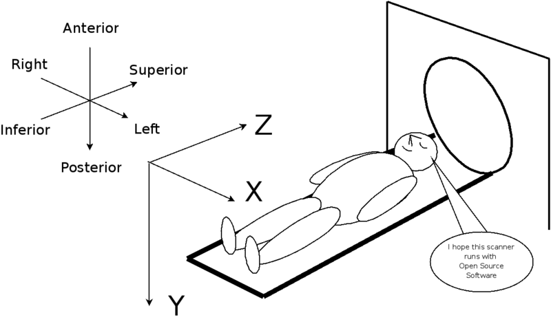
LPS Coordinate System (Kitware Attribution 2.5)
This gives the axis but not the origin. The origin is arbitrary. It's not important as long at it is coherent. You might have seen on TV or in movies, that when patients are being installed in a scanner, some red laser forming an X over their head or nose or belly button. This is what is used to indicate the origin to the machine. It is useful to indicate a reference point so then you can compare different datasets from different exams without too much registration. Anyway, the origin is a point in space where 0 is 0. That's it.
From that point on, all the coordinates you will find in DICOM will be based on this coordinate system and their units will be, expect in some cases, in millimeters. Let's suppose the head of the patient is at [0, 0, 0], a point at [12, 34, 41] is 10mm closer to the head than [12, 34, 51]. What an imaging system generates when it generates 3D data is a volume. This volume is independent of the patient. Of course, the purpose is to treat patient so the volume will most certainly contain the whole or part of the patient's anatomy but technically this is not a necessity and should never be taken for granted. This means that volume can be aligned with the patient axes or not and one should always be careful to never lose generality by assuming any link between the patient coordinate system and the volume coordinate system.
The volume coordinate system
A 3D volume is constituted of slices. Each slice is a 2D array of voxels and voxels are basically 3D pixels ; little square containing a value as acquired by the acquisition device. We will not be getting into all the possible storage variations. The most simple case is when each of those slices are stored into an individual DICOM file called an instance. This instance will contain all the necessary metadata to interpret the slice: the pixel data (size in bits, interpretation, number of rows and column) but also all the positioning information we need to precisely know where each pixel is positioned in the LPS system. These information comes from the Image Plane Module as defined in DICOM.

Slice Coordinate System
The slice coordinate system needs an origin, two axes (being a 2D coodinate system in a 3D vector space) and a unit (the voxel). In each DICOM instance representing a slice, the field (0020,0032) Image Position Patient will indicate the origin of the slice in the LPS coordinate system. It positions the whole slice in space. It indicates the center of the top-left voxel of the slice. There is an important subtility here: it is the center of the voxel, not the top-left corner of the voxel that this field relates to. A common mistake is to forget that. The orientation is given by (0020,0032) Image Orientation Patient. The field contain 6 numbers. The first 3 are the X-axis of the slice and the last 3 are the Y-axis. The SCS is still not defined though because Image Orientation Patient contains normalized vector, thus the "size" of the voxel is not yet integrated. For this, we need to consider that the unit of the coordinate system is the size of the voxel itself. This is provided by the (0028,0030) Pixel Spacing field. Here again, we talk about well-behaved DICOM files. But as it happens, Pixel Spacing is not always present or can be overidded by other fields. We assume, in our case, that Pixel Spacing gives us what we want. This field is an array of two numbers. The first is the distance between the center of each voxel of the slice and the voxel right below. The second is the the distance between the center of each voxel of the slice with the center of the voxel immediately to the right.

(0028,0030) Pixel Spacing
So how do we extend the slice coordinate to the volume coordinate system, including the Z axis? Well by first noting again that we are treating a particular case, which is the most common case: aligned slices. Indeed, each slice is independent, there is no guarantee that slices are parallel to each other or aligned. Some system will produce non-parallel slice for CBCT acquisition for example, or when the volume is skewed with respect to the axis of the slice. Let's not worry about that here. Our slices are considered all parallel and aligned and form a nice cube-like structure in space.
In that case, the origin of our volume is the origin of our first slice. The X and Y-axes of our volume is the X and Y-axes of the first slice. Simple enough. The Z-axis is the cross-product of X over Y: Z = X x Z. Z will then indicate the direction of the next slices in the volume. We will set the length of Z to the distance between the Image Position Patient of the first slice and the Image Position Patient of the second slice, so each increment in the Z direction gives use the next slice. So all in all [0, 0, 0] is the first voxel of the first row of our first slice. [1, 2, 3] is the second voxel of the third raw of the fourth slice of the volume.
Convertion
And Now the final step. We will create the homogeneous matrix representing the volume coordinate system and let the math do the work. This matrix will help us know:
- The coordinate in LPS of any voxel
- The index of a voxel at a particular place in space

The volume homogeneous matrix
This is our Ba matrix. In input it will take a vector containing the indices of a voxel in the volume and will give its position in space in output. Invert the matrix and you will get the opposite transformation.
The camera and its coordinate system
The final piece of the coordinate system puzzle is the camera. The pinhole camera model has been the bread and butter of 3D computer graphics and we will not go into much detail here as this case has been covered many times over. You can try to wrap your head around the Wikipedia page but I find the explanation from scratchapixel more intuitive.
Our camera model is pretty simple. It relies on two points and a vector: eye point, look point and the up vector. The camera plane is the plane going through the look point and perpendicular to the camera direction indicated by the vector (look point - eye point). The plane segment, called the camera plane, is delimited by the Field Of View (FOV) which, in our case, will be defined as the height of the camera plane in millimeters. Note that the FOV is usually defined as the diagonal. To simplify here, we consider that the camera plane as a square (FOVx = FOVy). The up vector gives us the orientation of the camera plane. Rotating the camera is then a matter of rotating the up vector:

The camera model
But keep in mind that the pinhole camera presented all over the internet is usually meant as a projection of a 3D space into a plane. In the case of an MPR rendering, the camera is going to be used differently. The camera plane is going to cut through the volume and each pixel of the camera is going to be mapped with a volume voxel:

The camera plane cut the volume
The origin
The coordinate system of the camera is starting to appear clearly. Let's start with the origin. The top-left corner of the camera plane can be obtained from the look point and moving it along the plane following the up vector direction by FOV/2 mm will position it at the top edge. We need now to move it to the left again by FOV/2 mm and that's it. But how to know what is left? We have the up vector giving us up, but no left vector. We are going to create one. More precisely, we are going to create a "right" vector which is the cross product of the direction vector (look point - eye point) by the up vector: right = (look-eye) x up. Moving the look point to the left just mean moving it along the -right vector.
The base
We will create a coordinate system which as simple as possible and set aside efficient computation aside. The base of our coordinate system will encompass the whole camera plane. It means that between 0 and 1 you will live in that segment. Outside of that range, you are out of the segment. This greatly simplified the explanation but will lead us to perform some unnecessary costly floating point arithmetic, especially division, but efficiency is not the point of this series of articles anyway.

The camera coordinate system
Those axes then are pretty easy to define. The X-axis is the normalized right vector multiplied by the FOV (remember that the camera plane is a square so its width and height is equal to the FOV). The Y-axis is the normalized up vector multiplied by -FOV. "Minus" because the Y-axis direction is opposed to the up vector.
The matrix
"What is the matrix?". Well, we have all the elements to build it now. Let's define:
- X = -FOV * |up|
- Y = FOV * |right| and
- O = look + FOV / 2 * |up| - FOV / 2 * |right|

The camera homogeneous matrix
Note that although our plane is a 2D space, it remains that we are still situated in a 3D space so the matrix also as a Z component which is the null vector here. And our point in our camera plane are still homogeneous 3D points so if we were to represent the look point for example, it would look like: [0.5, 0.5, 0, 1].
Here again we can use this matrix to go to and from the patient coordinate system. So we are now free to hop from the camera to the patient to the volume coordinate system freely and very easily by multiplying matrices and their inverses with ease.
Conclusion
We are getting close. We have all the tools now to render an arbitrary plane in our volume. We just need to put it all together: reading the DICOM, extracting the pixels, positioning the plane and rendering our image. From all the complexity of that subject, the resulting code will be deceptively simple because the underlying mathematical operation is simple. The complexity is in the details.
Next the actual rendering.