From DICOM to MPR (part 2)
The format
This is the second part of 5 parts series. Link to part 3.
So what is DICOM? According to David Clunie, in his presentation "DICOM: Overview and historical perspective", it is:
- Application/modality specific Information Object Definitions (IODs) for data sets
- A standard file format in which to store data sets
- Data sets for images, parametric maps, segmentations, spectra, waveforms, point clouds, meshes, contours, annotations, transformations, reports, protocols, plans, ... anything image-related
- Standard protocols to send, query for and retrieve data sets (and other things)
- A conformance documentation mechanism
- A data dictionary (elements, what they mean, how they are encoded)
- A controlled terminology (standard codes with standard definitions)
- Value sets (which standard codes to use in which contexts)
As you can see, DICOM is vast. We won't become DICOM experts on this blog. Our purpose remain modest: being able to extract images and display them. For this, we will not be digging into the networking protocols, how to store a mesh or all the "standard codes". We just need to know enough of the format for our goal: render an MPR image (sordid details following).
The first ARC-NEMA standard purpose was to transmit data from a computer to another. At that time, Ethernet didn't exist and everything had to be invented. So the ARC-NEMA joint committee designed a special type of connector and associated protocols to transmit information. It would be a 50 pin 16 bits parallel interface which would transport data under the form of commands themselves containing pairs of tag/value. The tag would indicate the type of information to follow. Each tag would be composed of a Group, an Element and a length of data, then the data would follow.
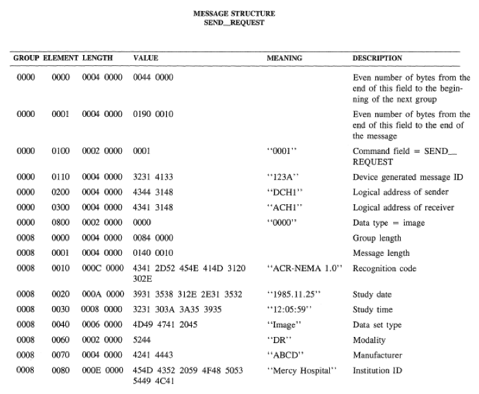
A message structure as described in D. Clunie's presentation.
And so DICOM evolved from that basic principle: pairs of tag-values. Not necessarily the most elegant format but the best that they could come up at the time with the limited computing resources they could muster. One of the difficult aspect of DICOM is its variability. It has been used for 30 years and has not always been perfectly respected by manufacturers and has also evolved into different variants. Some DICOM files are little endian, some are big endian. Some files will have implicit value representation, some others won't. Some will have a header, others won't. In the course of this article we will always take for granted a modern, nicely formatted file. We let real world projects deal with the nasty variations.

Data elements.
Each tag represents a specific field and is described in the DICOM Data Dictionary (be warned, this is a big page!). I talked about "value representation" (VR). This is the type of a specific field. For example, the VR for the tag (0008,0020) Study Date is DA. Looking at the definition page for VR on the NEMA site, DA is Date. It has a specific format and the page describes how to parse it to extract the information. It says: "A string of characters of the format YYYYMMDD; where YYYY shall contain year, MM shall contain the month, and DD shall contain the day, interpreted as a date of the Gregorian calendar system.". So the data will be contained in 8 characters (or bytes) which will represent numbers associated with a year, a month and a day. If we look at the earlier example, we can see the study date is formatted this way:
      │GRP.│ELT.│LENGTH   │DATA                    │
      ├────┼────┼─────────┼────────────────────────┤
      │0008│0020│000A 0000│3931 3538 312E 2E31 3532│
In the first two versions of the DICOM standard, which was called ARC-NEMA at the time, groups had a meaning. 0008 was "Identifying Information". I couldn't find any definition of individual groups in DICOM v3. In that version it seems, groups have lost their meaning and can be considered as part of the identifier of a tag.
0020 is the element and represent the study date within the "Identifying Information" group.
000A is the data length which in decimal is 10 bytes. "But wait! Didn't the standard specified a length of 8 bytes for a date". That's because you didn't read the fine prints. Right below: "The ACR-NEMA Standard 300 (predecessor to DICOM) supported a string of characters of the format YYYY.MM.DD for this VR. Use of this format is not compliant.". This is the story of DICOM. It's not compliant but still described in the standard and is actually used. The standard is just paper. You will have to adapt to what you will find in the field.
Finally, our 10 bytes of data: 3931 3538 312E 2E31 3532. Armed with your ascii table you will decode the message:
      Hex    Char
      -----------
       2E    .
       ...
       30    0
       31    1
       32    2
       33    3
       34    4
       35    5
       36    6
       37    7
       38    8
       39    9
       ...
So: 9158 1..1 52. Now that is a strange date. But remember that DICOM does
not specify an
endianess. Your file can be little or big endian and in our case, it
probably is little-endian:

A practical example
Let's put all this knowledge in application. We will load a DICOM file in our browser, and dissect it until we find the study date. First, load the dataset as an TypedArray:
  const response = await fetch('http://site.novidee.com/assets/IM0257_0');
  const dataset = new Uint8Array(await response.arrayBuffer());
Now dataset contains our DICOM file. Note that DICOM files can either contain one CT slice or multiple CT slices (a whole volume). The latter would be called a multi-frame DICOM file. This is not our case here, to keep it simple, we have 1 DICOM file = 1 slice. To process that file we will need to access individual fields (the value part of the pair tag/value). For that purpose, we will write a nextTag and getTag function which will walk the file, field by field, until it find the requested tag and returns its value:
// nextTag is called by getTag.
function nextTag(dataset, offset) {
  const tag = dataset.slice(offset, offset + 4);
  offset += 4; // Skip tag
  const VR = String.fromCharCode.apply(null, dataset.slice(offset, offset + 2));
  offset += 2; // Skip VR
  if (['OB', 'OD', 'OF', 'OL', 'OW', 'SQ', 'UC', 'UR', 'UT', 'UN'].includes(VR)) {
    // These VR types handles themselves differently. They have 2 reserved bytes
    // that need to be skipped and their data length is on 4 bytes.
    offset += 2 // Skip reserved byte
    if (VR === 'SQ') { // Sequence are s special type within those specials types... yikes.
      // See http://dicom.nema.org/dicom/2013/output/chtml/part05/sect_7.5.html on
      // how a sequence look like in a DICOM file. Let's throw an error for now.
      throw new Error('Oops, we do not deal with SeQuence fields for now... :/');
    }
    length = dataset[offset] +
      (dataset[offset + 1] << 8) +
      (dataset[offset + 2] << 16) +
      (dataset[offset + 3] << 24);
    offset += 4; // Skip length
  } else {
    // The tag with "regular" VR have 2 bytes long datalength field.
    length = dataset[offset] + (dataset[offset + 1] << 8);
    offset += 2; // Skip length
  }
  const dataOffset = offset;
  return {
    tag, VR, length, dataOffset
  };
}

function getTag(dataset, tag) {
  // Convert the convenient string format to a binary array.
  // Flipping the element to match the endianess of the DICOM file.
  const binTag = [
    parseInt(tag.substring(2, 4), 16),
    parseInt(tag.substring(0, 2), 16),
    parseInt(tag.substring(6, 8), 16),
    parseInt(tag.substring(4, 6), 16),
  ];
  // Assuming a nice DICOM file. We skip the first 128 bytes, then the "DICM"
  // flag. Then will fast forward the header (assuming an explicit VR type)
  let offset = 128 + 'DICM'.length;
  let dataElement;
  do {
    dataElement = nextTag(dataset, offset);
    offset = dataElement.dataOffset + dataElement.length;
  } while (
    // While we don't reach the end of the file
    offset < dataset.length &&
    // and as long as we have not found our tag, we will jump to the next one.
    !(dataElement.tag[0] === binTag[0] &&
      dataElement.tag[1] === binTag[1] &&
      dataElement.tag[2] === binTag[2] &&
      dataElement.tag[3] === binTag[3])
  );
  // Return a slice of the data containing the value. Up to the called
  // to format to the proper type.
  return dataset.slice(dataElement.dataOffset, dataElement.dataOffset + dataElement.length);
}
Note that we skip 128 bytes at the beginning of the file in the addition of the "DICM" string. Again, most modern properly formatted DICOM files follow that convention. Others don't... You've been warned. Now let's try it with the Study Date field on the dataset we loaded previously:
  > console.log(String.fromCharCode.apply(null, getTag(dataset, '00080020')));
  20090610
That's it, you got a date! In term of performance, this function is a joke, rereading the same field again and again, but it is simple and it does the job. Good enough for now. By the way, you can copy paste all this code in your browser if you want to try it yourselves. I don't guarantee that I will host that DICOM file forever so feel free to change the URL to any "regular" CT DICOM file you will find on the interweb from a server accepting CORS requests. Otherwise pyton3 -m http.server is your friend.
From DICOM to an image
This was a deep dive into the entrails of DICOM. We will now use that knowledge to render a simple DICOM image into a canvas. But how to do that? First of all, the steps needed to render an image from a DICOM file depends on the type of image contained. As explained in the first part, DICOM files can contain various type of data, most of them are images but not only. And those images can be of very different types. From a raw CT slice to a screenshot, you will have to adapt the steps you need to take to render that image.
Bits Storage
The first important information that you will need to retrieve is how the pixel are stored in the DICOM file. They can be stored in 8 bits or 16 bits (or any number of bits in fact). They can be represented as signed or unsigned integers or even floats. In order to know the storage profile of our image we will need to read the following fields:
- (0028,0100) Bits Allocated and (0028,0101) Bits Stored: Bits Allocated will tell you how many bits is using each pixel on the disk. For example, a Bits Allocated to 16 and 10 pixel in your file will use 160 bits. However, less bits might actually be used. If the range of data can be expressed in less than 16 bits (for example from -1000 to +3000) only 12 bits might be used. In that case Bits Stored will be 12. The 4 additional bits will just be padding.
- (0028,0103) Pixel Representation: Indicates if the data is signed (1) or unsigned (0).
function twoBytesToNumber(arrayBuffer) {
  return (arrayBuffer[1] << 8) | arrayBuffer[0];
}
Then read those three fields:
  > console.log('BitsAllocated', twoBytesToNumber(getTag(dataset, '00280100')));
  16
  > console.log('BitsStored', twoBytesToNumber(getTag(dataset, '00280101')));
  12
  > console.log('PixelRepresentation', twoBytesToNumber(getTag(dataset, '00280103')));
  0
So we conclude that, in that particular file, data is unsigned and pixels are stored on 12 bits but we will need to count 16 bits for the total pixel buffer to read.
Modality LUT
When an acquisition machine stores data, it does it in a opaque way. Reading the data stored would not help you know if you are looking at bone, skin or lung. This allow various manufacturer to store raw data from their machine without worrying too much about interoperability. However, to ensure interoperability, manufacturer will need to provide parameters that will allow an external party to convert that opaque internal representation to a universal format. For example, Godfrey Hounsfield invented a scale that would map unique value to material types. This is called the Hounsfield scale. Certain value on this scale represent the density of well known material. -1000 is the density of Air, cancerous bone is between 300 and 400 and muscle is between 35 and 55. DICOM defines a way to convert the internal opaque representation to Hounsfield Unit (HU) called the Modality LUT. You will hear a lot about LUT (Look Up Table) when working with DICOM files. Initially meant as an array mapping between values, they have been, in the context of DICOM, generalized to describe functions that performs an intensity transformation. In the simplest case, a Modality LUT is a linear affine function: 𝒚 = 𝐚 𝑥 + 𝐛. 𝐚 is the slope (RescaleSlope 0028,1053) and 𝐛 the intercept (RescaleIntercept 0028,1052). After applying that function you will get values in HU. Note that HU are not the only form of intermediary representation, DICOM defined multiple types of unit depending on the modality.
VOI LUT
Now that our pixels are expressed in a universal unit we need to display them on the screen. As it happens, the human eyes is not able to distinguish between more than ~100 different shades of gray. So displaying pixels which can range between -1000 and 3000 will not help your diagnosis. So you will want to reduce that range to an appropriate displayable 8 bits range (0-255). But that means you will loose details. Compressing a 12 or 16 bits range to 8 bits will, inevitably, result in information loss. But that is not necessarily a problem. Because doctors will only want to see certain types of tissue. Even if your range can express values from air (-1000) to brass (+30000), you might be only interested in lung tissue (-700 to -600) or gray matter (+37 to +45). In order to "zoom" into that value range and map it to the display range (0-255) you will apply a windowing technique. Windowing is a way to linearly map a range to another.

The Windowing operation
In this, somewhat crude, illustration, you can see that the input range (the x axis) is mapped onto the output range (the y axis). Every value below 100 will be set to 0 and every value above 200 will be saturated to 255. The range in between 100 and 200 will be distributed linearly on the output range. For example, the value 150 (in the middle of the input range) will be mapped to 128 (the middle of the output range). What defines a window is its center and its width. The center will slide the window along the input range and the width defines how much of the input is mapped.
Like the modality LUT, the Value Of Interest (VOI) LUT can take different form: an actual Look Up Table (called sequence), a sigmoid function or the most common case, a simple linear function. The illustration above is for a linear function which is entirely defined by the following two parameters:
- The WindowCenter (0028,0150)
- The WindowWidth (0028,0151)
Rendering pipeline
When those steps are combined, it gives that nice rendering pipeline:

The Rendering pipeline
Armed with the getTag and twoBytesToNumber functions, you can now load all the data you need:
      const bitsAllocated = twoBytesToNumber(getTag(dataset, '00280100'));
      const rescaleIntercept = parseInt(String.fromCharCode.apply(null, getTag(dataset, '00281052')), 10);
      const rescaleSlope = parseInt(String.fromCharCode.apply(null, getTag(dataset, '00281053')), 10);
      const windowCenter = String.fromCharCode.apply(null, getTag(dataset, '00281050')).split('\\').map(parseInt)[0];
      const windowWidth = String.fromCharCode.apply(null, getTag(dataset, '00281051')).split('\\').map(parseInt)[0];
      const rows = twoBytesToNumber(getTag(dataset, '00280010'));
      const columns = twoBytesToNumber(getTag(dataset, '00280011'));
      if (bitsAllocated !== 16) {
        throw new Error('Oh no, not a 16 bits dataset!');
      }
      const pixels = new Uint16Array(getTag(dataset, '7fe00010'));
First, note that RescaleSlope and RescaleIntercept are store with a value representation of DS (Decimal String). You have to convert the data extracted to a string and then apply parseInt. Then, WindowCenter and WindowWidth are also stored as DS but with a value multiplicity of 1-n. That means those fields are basically arrays, they can store between 1 to n values. This is all visible on the NEMA website for DICOM. If you look at the string retrieved from WindowCenter for example:
    > String.fromCharCode.apply(null, getTag(dataset, '00281050'));
    "00100\\00100 "
The array is represented by values separated by '\\'. That is why we split by '\\'. In our case, we immediately select the first value to stay simple. In practice, the different values correspond to different profiles, meaning different type of "views" you can offer. The different values of the array are explained by the field (0028,1055) Window Center & Width Explanation Attribute.
Finally Rows (0028,0010) and Columns (0028,0011) are the dimension of a slice. Width and height basically.
We've loaded the pixels and the parameters we need. Now we will apply the modality LUT, which will give us hounsfield units, and then the VOI LUT, which will give us greyscale values ready to be loaded onto a canvas:
      const imageBuffer = new Uint8ClampedArray(pixels.map(pixel => {
        // Apply modality LUT
        const hu = pixel * rescaleSlope + rescaleIntercept;
        const lowerBound = windowCenter - windowWidth / 2;
        // Apply VOI LUT
        const higherBound = windowCenter + windowWidth / 2;
        if (hu < lowerBound) {
          return 0;
        } else if (hu > higherBound) {
          return 255;
        } else {
          return (hu - lowerBound) / (higherBound - lowerBound) * 255;
        }
      }));
      // Convert our greyscale image to an RGBA (see canvas API on MDN).
      const imageData = new ImageData(columns, rows);
      imageBuffer.forEach((pixel, index) => {
        imageData.data[index * 4    ] = pixel; // R
        imageData.data[index * 4 + 1] = pixel; // G
        imageData.data[index * 4 + 2] = pixel; // B
        imageData.data[index * 4 + 3] = 255; // A (255 is completely opaque)
      });
      const canvas = document.createElement('canvas');
      canvas.width = columns;
      canvas.height = columns;
      const ctx = canvas.getContext('2d');
      ctx.putImageData(imageData, 0, 0);
      // You should now see an nice image in your page ! :)
      document.body.appendChild(canvas);
Et voilà. Your image should be appended to you document body, thus visible in your page. Note that we had to convert the greyscale image resulting from the VOI LUT windowing to RGBA, but this has nothing to do with DICOM. It's just that the canvas API, which I strongly advise you to master, only accepts RGBA when putImageData is used.
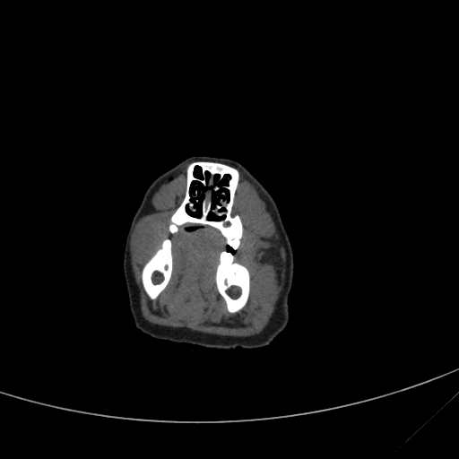
The rendered slice. Coudn't tell you what part of the anatomy this is!
Conclusion, for now...
All in all, this was a pretty beefy blog post. A lot of moving parts and also a deep dive into DICOM which might leave you dizzy a little bit. But stay strong, on the next part of this four parts series, we will have a look at a less technical and a more mathematical aspect of DICOM: coordinate systems. Onward and upward !
A word of warning. DICOM is a complex beast and, in this example, we have oversimplified things a bit in order to keep the article engaging. But if you were to write a proper DICOM viewer, there are many things that you would have to take into consideration. What about the photometric interpretation of the pixels? Is it MONOCHROME1 or MONOCHROME2? Is it a color image? Does the VOI function is LINEAR or LINEAR_EXACT? What is the "spacing" of each of the pixel? etc, etc. Additionally, the code presented here is in no way optimized. Quite the contrary, performance has been sacrificed to keep it simple. Processing DICOM image can be quite slow due to the nature of the format, the size of the images and the processing applied to them. If you were to write a "real" viewer in Javascript, there would be a lot of work just to make it usable.
Next some geometry reminders.